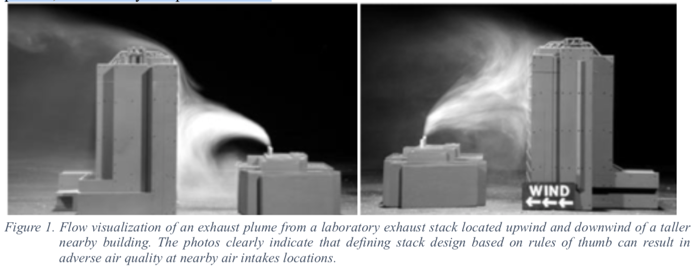
A laboratory exhaust system is designed to not only remove contaminated air from within the laboratory and fume cupboards, but it also serves to safely discharge the exhaust away from the building, so that hazardous and odorous fumes do not re-enter through air intakes or affect surrounding sensitive locations (receptors). This is achieved through proper combination of stack height and exhaust discharge momentum, i.e. plume rise. With shorter stack heights, greater plume rise, and thus more fan energy is needed to transport the exhaust safely away from the building. Alternately, if the exhaust stack is taller, less plume rise and less fan energy is required.
Often the design of laboratory exhaust stacks is based on rules of thumb described in various standards and best practices guides1,2,3,4; which typically define the minimum stack heights (3 m to 1.25 times the height of the building) and exit velocities (10 m/s to 15 m/s). Unfortunately, stack height and exit velocity alone is not sufficient to define, whether or not acceptable air quality will be present, at all nearby receptor locations.
Rather than using rules of thumb, the proper combination of stack height and exhaust discharge momentum (energy) should be determined using an engineering analysis technique called exhaust dispersion modeling. Dispersion modeling is used to predict concentration distributions at sensitive locations in the surrounding area as a function of wind speed and wind direction. An exhaust system is considered acceptable when the maximum predicted concentration is less than or equal to a design goal that is developed to ensure that the effluent concentrations remain below published health limits and odor threshold values6,7,8.
At wind directions and wind speeds where the predicted concentrations are lower than the design goal, it is often possible to reduce the discharge momentum and still achieve the design goal, while saving significant energy. To define the most energy efficient exhaust system, physical dispersion modeling (i.e., wind tunnel modeling) should be utilized.
Defining an Acceptable Design Goal for Re-entrainment of Laboratory Exhaust!
To evaluate air quality acceptability, dispersion modeling techniques are used to predict the maximum concentration of an exhaust plume that is present at nearby receptor locations. However, this information is not useful unless some maximum acceptable concentration, or design goal, is specified. The question of air quality acceptability can be expressed as:
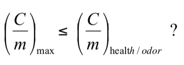
where (C/m)max is the maximum predicted normalized concentration at a receptor location (air intakes, operable windows, pedestrian areas, etc.), (C/m)health/odor is the normalized health limit or odor threshold concentration of any emitted chemical. The left side of the equation, (C/m)max, is only dependent on external factors such as the exhaust stack operating parameters, receptor locations, and atmospheric conditions. The right side of each equation is related to the emissions and is defined as the ratio of the health limit or odor threshold (μg/m3) to the emission rate (g/s). Therefore, a highly toxic chemical with a low emission rate may be of less concern than a less toxic chemical emitted at a very high rate.
In practice, a chemical inventory for each exhaust type is examined to determine the appropriate values of (C/m)health and (C/m)odor for any released chemicals. Dispersion modeling is performed to determine (C/m)max for the various stack designs evaluated. Those designs that yield concentrations at or lower than the design goal, i.e., (C/m)max ≤ (C/m)goal, are considered acceptable.
Dispersion Modeling Methods!
Concentration predictions (C/m) at sensitive locations can be accomplished with varying degrees of accuracy using three different types of studies:
- A full-scale field monitoring;
- A numerical modeling study; or
- A reduced scale wind-tunnel study.
Full-scale Field Monitoring!
A full-scale field monitoring program involves releasing a tracer gas from within the exhaust system and measuring concentration at downwind receptor locations. Although it may yield the most accurate predictions of exhaust behavior, it is often expensive and time consuming to execute. In addition, it can only be conducted for existing laboratory facilities. If the nature of the study is to estimate maximum concentrations for several stacks at several locations, many years of data collection may be required before the maximum concentrations associated with the worst-case meteorological conditions are measured.
Numerical Dispersion Modeling
Gaussian based Analytical Models
Downwind concentrations of an exhaust plume can be calculated using the Gaussian based analytical dispersion model presented in the ASHRAE Handbook − HVAC Applications4 and in the ASHRAE Laboratory Design Guide5. The model is designed for an isolated rectangular building with roof top stacks and does not take into account effects from neighboring buildings, elevated terrain, or vegetation that is sufficient enough to impact the air flow along the top of the roof. The model assumes that the emissions are not caught within a weak recirculation region downwind of the building, so it should not be used for ground level emissions with stack heights below an adjacent roof top.
When properly applied, the ASHRAE dispersion model is designed to be conservative (i.e., underestimate dilution/overestimate concentrations). However, it has been found to be non- conservative when a building corner is directly upwind of the direct line between the stack and downwind air intake9, or when the stacks are located within a screen wall10. Furthermore, the dispersion model does not take advantage of the reduction in concentrations at air intakes that are “hidden” from the exhaust stack11. Thus, when using the ASHRAE dispersion model, care should be taken to make sure that the model is applied appropriately.
Computational Fluid Dynamics
Computation Fluid Dynamics (CFD) has been used for quite some time to successfully model internal flow fields within such areas as laboratories and vivarium. As such, there is a natural tendency to attempt to use the same model for external air flow to model the performance of laboratory exhaust stacks. Unfortunately, the simulation techniques used for indoor simulations are ill suited for modeling atmospheric turbulence. Since the dispersion of an exhaust plume is directly related to the atmospheric turbulence, even small errors in the simulation of turbulence can result in large errors in the predicted downwind concentrations.
Current research into the use of CFD models for dispersion modeling has indicated that non- steady simulations, such as Large Eddy Simulation (LES), show the most promise. However, LES models are more difficult and time consuming to run and even the results of LES simulations should undergo validation to verify their accuracy12.
At this time, due to the constraints described above on the use of CFD for laboratory exhaust dispersion, it should be considered more of a research tool than a design tool that can be used for properly sizing laboratory exhaust systems.
Wind Tunnel Dispersion Modeling
Wind-tunnel modeling is often the preferred method for predicting maximum concentrations for stack designs and locations of interest, and is recommended because it gives the most accurate estimates of concentration levels in complex building environments4. A wind-tunnel modeling study is like a full-scale field study, except it is conducted in a controlled environment before or after a project is constructed. Typically, a scale model of the building under evaluation, along with the surrounding buildings and terrain within a 300-meter radius, is placed in an atmospheric boundary layer wind tunnel. A tracer gas is released from the exhaust sources of interest, and concentration levels of this gas are then measured at receptor locations of interest and converted to full-scale concentration values. Next, these values are compared against the appropriate design criteria to evaluate the acceptability of the exhaust design. ASHRAE4 and the EPA13 provide more information on scale- model simulation and testing methods.
Wind-tunnel studies are highly technical, so care should be taken when selecting a dispersion modeling consultant. Factors such as past experience, proper calibration of the wind tunnels13, and technical qualifications of the staff are extremely important.
Energy Saving Laboratory Exhaust System Strategies!
Manifolded Laboratory Exhaust Systems
Combining exhausts into a common exhaust system, either by manifolding exhausts or with very close grouping of stacks (stacks must nearly touch for the exhaust plumes to merge under all wind directions), will enhance the rise of the exhaust plume, reducing downwind concentrations for receptors below the height of the stack. Close grouping of stacks can be used for specialty exhausts, such as Perchloric Acid and Radioisotope, which cannot be manifolded because of their chemical nature. Manifolding or combining exhausts can generally create greater plume rise than installing an exhaust nozzle on a stack serving a single laboratory chemical hood.
Manifolding of exhausts can also provide some internal dilution of fume cupboard exhausts when the majority of chemical emissions are from an upset condition or large release from a single laboratory chemical hood. Such upset or large release conditions are the primary cause of odor complaints and potential health effects.
Typically, laboratory exhaust manifolds are served by multiple exhaust fans. The fans are often sized such that the building exhaust requirements can be met with one or more of the exhaust fans turned off. In this case, the manifolded system provides redundancy in the case of a fan failure. This makes a manifolded system safer for the laboratory occupants than an individual fume cupboard exhaust system. Overall, a manifolded system provides the following advantages3:
- Lower capital and operational costs;
- Fewer exhaust stacks;
- Greater adaptability of design;
- Simpler effluent treatment;
- Added dilution and momentum;
- Reduced maintenance costs;
- Fan redundancy
- Potential for energy recovery;
- Fewer roof penetrations; and
- Reduction in the total volume flow rate requirements.
Variable Air Volume Laboratory Exhaust Control Strategies
Designing a laboratory to utilize a Variable Air Volume (VAV) exhaust system allows the exhaust ventilation system to match, or nearly match, the supply ventilation airflow requirement of the building. This allows the designer to take full advantage of energy-saving opportunities associated with employing various strategies to minimize airflow requirements for the laboratory. However, just as arbitrarily reducing the supply airflow may adversely affect air quality within the laboratory environment, blindly converting an exhaust system to VAV without a clear understanding of how the system will perform can compromise air quality at nearby sensitive receptor locations (e.g., air intakes, operable windows, plazas, etc.). Therefore, before employing a VAV system, the potential range of operating conditions should be carefully evaluated through a detailed dispersion modeling study, as described above. Since the nature of these assessments is to accurately determine the minimum volume flow requirements for the exhaust system, the preferred method is the use of physical modeling in a boundary-layer wind tunnel. Numerical methods can be used, but these will more often than not, result in higher minimum volume flow rates when properly conducted and the resulting energy savings potential will be reduced.
Two different strategies that can be used for operating VAV laboratory exhaust systems are described below.
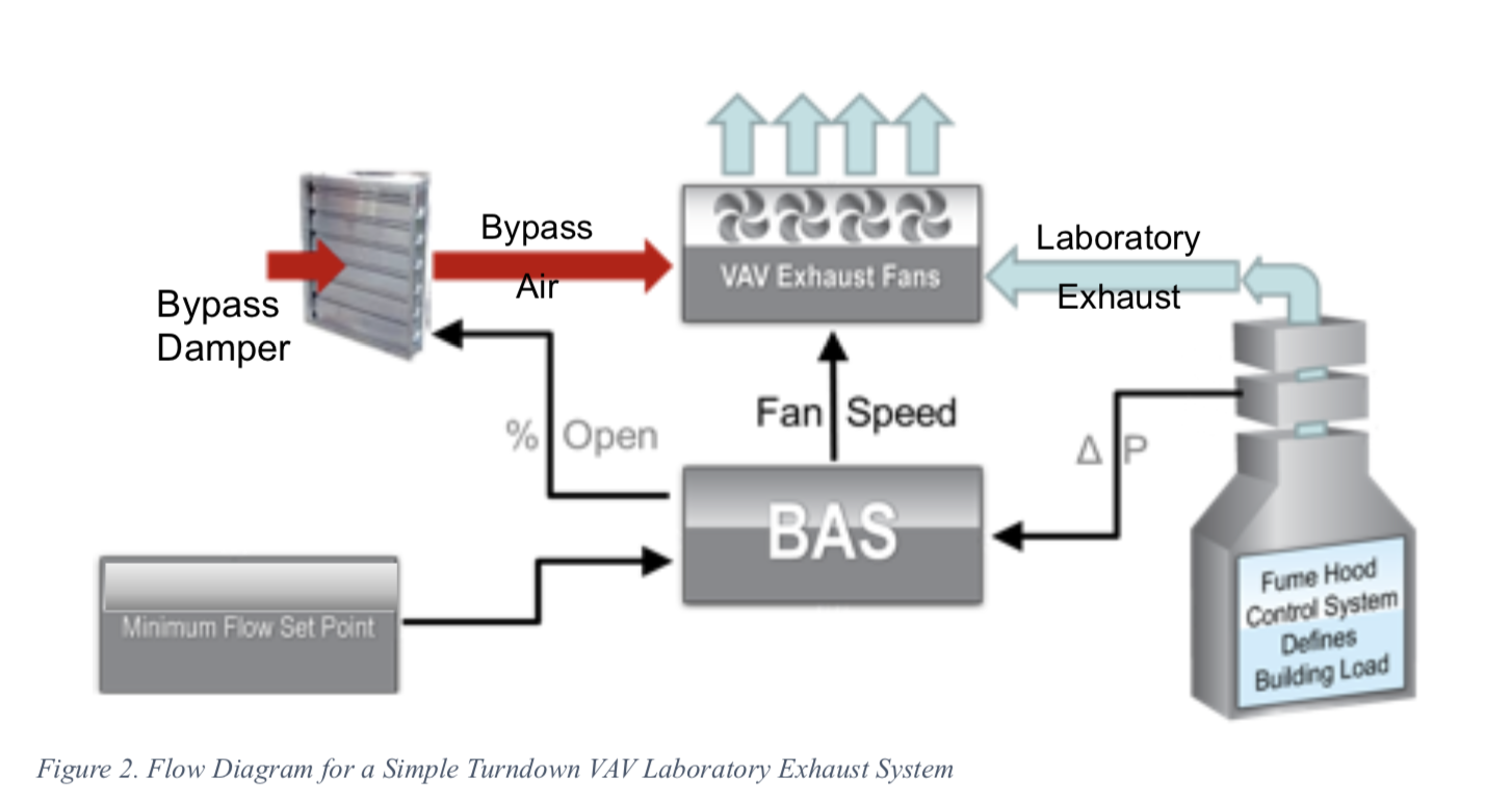
Strategy 1: Simple turndown VAV Laboratory Exhaust System!
In a simple turndown VAV system, the exhaust flow is based on the greater of two values: the minimum air quality set point and the building’s ventilation demand. The minimum air quality set point is defined as the minimum volume flow rate/exit velocity/stack height needed to provide acceptable air quality at all sensitive receptor locations under worst-case wind conditions, as defined in the dispersion modeling assessment. During the assessment, when a simple turndown VAV system is to be employed, the stack design often focuses on the minimum potential volume flow rate for the laboratory building rather than the maximum value as evaluated for a constant volume exhaust system. The preference is to design a simple turndown system where the exhaust fans are able to fully adjust the volume flow rate to meet both the minimum and maximum laboratory exhaust demands. This results in a system that responds quickly to pressure excursions and eliminates the need for bypass dampers. This can often be achieved by evaluating the number of stacks feeding off of each plenum and the subsequent height requirements needed to fully eliminate the need for bypass air through a combination of VAV control and staging of fans.
Strategy 2: Wind Responsive VAV Laboratory Exhaust System!
If the simple turndown VAV system does not result in minimum volume flow rates that are equal to, or lower than, the building ventilation demand, or, if the required stack heights to achieve these minimum volume flow rates are too tall, further optimization is available by applying a wind responsive VAV laboratory exhaust system.
In this strategy, a local anemometer is connected to the building automation system (BAS) and the minimum required exhaust flow rate is varied based on current wind conditions (direction and speed). When the current wind speed and/or wind direction does not correspond with worst-case conditions (as assumed in the simple turndown strategy), the exhaust system may be turned down to more closely match the building demand. Essentially, the minimum set point is specified for each wind direction/speed combination. This usually results in air minimum volume flowrate set points that are well below building demand for many wind conditions, allowing the entire ventilation system to operate at optimum efficiency.
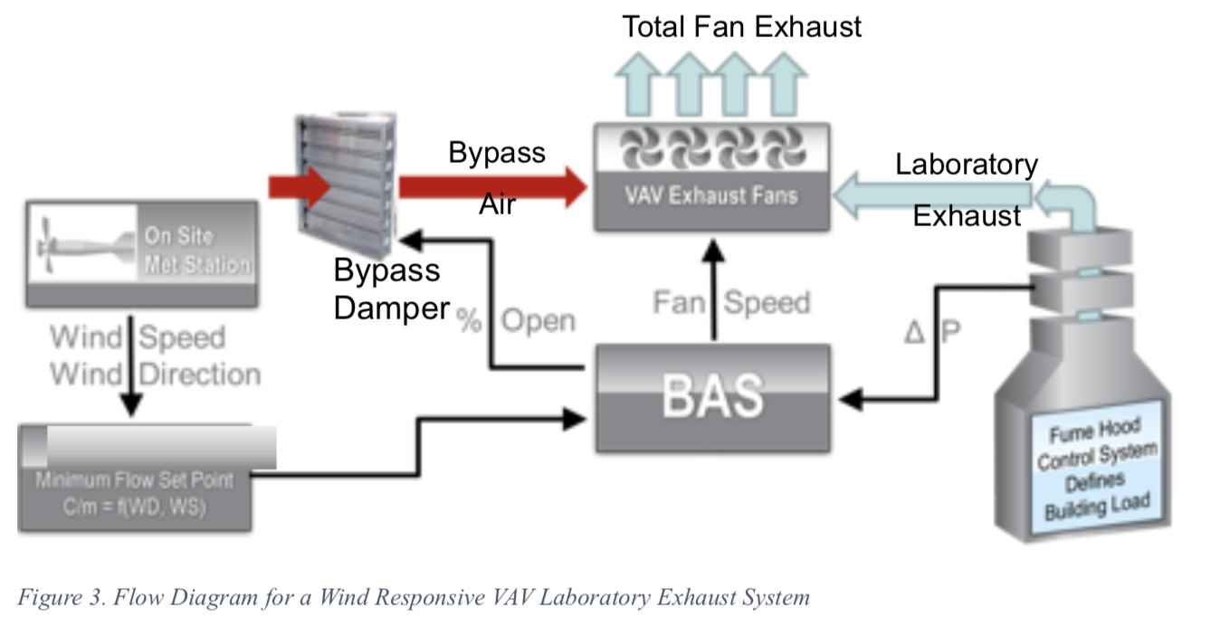
This strategy requires physical exhaust dispersion modeling in a wind tunnel, as most numerical dispersion models do not provide off-axis concentration predictions. Minimum volume flow rate set points as a function of wind direction (WD) and wind speed (WS) require concentration predictions at all sensitive locations (receptors) for all wind directions, wind speeds, stack heights, and exhaust flow parameters.
Summary and Conclusions!
An accurate assessment of exhaust dispersion can be used to provide exhaust/intake designs that are optimized for safety and energy consumption. No matter what type of exhaust system is used, the important design parameters are physical stack height, volume flow rate, exit velocity, expected pollutant emission rates, and concentration levels at sensitive locations. The overall performance should be evaluated using the appropriate criterion that ensures acceptable concentrations at sensitive locations. When employing a VAV laboratory ventilation supply system for the laboratory, the design team should strongly consider opportunities to include VAV laboratory exhaust systems as well, to fully realize the energy savings potential of VAV control. However, blindly applying VAV to the laboratory exhaust system using “rule of thumb” operating parameters can be detrimental to the air quality at air intakes and other locations of concern. Therefore, a dispersion modeling assessment should be conducted to define acceptable minimum volume flow rates. Any implementation of a VAV exhaust system should include a building automation system designed to handle the appropriate control logic. In addition, commissioning of the system should include the full range of operating conditions.